Chapter 2 Methodological framework
n this chapter we briefly introduce some of the key concepts related to the methods we used in our work. More precisely, we cover the technical concepts related to speech production mechanisms, to electromyography and to our statistical approach. Finally, we give an overview of the following chapters.
2.1 Biomechanical aspects of speech production
2.1.1 Vocal apparatus
Speech production requires the involvement of more than 100 muscles in the face, the neck and the chest (Simonyan & Horwitz, 2011). The activity of these muscles is coordinated to produce an air flow moving from the lungs to the oral and nasal cavities, via the trachea, the larynx and the pharynx (see Figure 2.1). Broadly speaking, speech production can be said to consist essentially in i) phonation, which refers to the control of the air flow and to the vibration of the vocal folds and ii) articulation, which refers to movements of the articulators. The action of the articulators (e.g., lips, tongue) is to shape the oral and nasal cavities, resulting in modifications of the sound waves and in the production of different vowels and consonants.
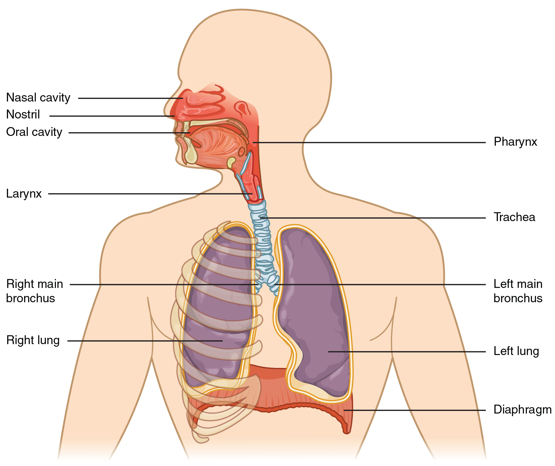
Figure 2.1: Human respiratory and phonatory system. Figure from the OpenStax Textbook. Download for free at .
The characteristics of the vocal folds (e.g., their length or thickness) influence what is known as the fundamental frequency (or F0) of the speech signal, which in turn determines the perceived pitch of the voice. The speech signal can be further decomposed in resonant frequencies or formants. We can relate changes in the state of the articulatory system with changes in the formant (and especially the F1-F2) space (see Figure 2.2). Indeed, the frequency of the first formant (F1) is mostly determined by the height of the tongue body (or rather by the aperture of the oral cavity) whereas the frequency of the second formant (F2) is mostly determined by the frontness/backness of the tongue body. For instance, when producing the /u/ vowel, the oral cavity is in a close position and the tongue lies in the back of the oral cavity (and the lips are rounded). However, when producing the /a/ vowel, the oral aperture is larger (and the lips are widely opened).
Figure 2.2: Illustration of the vocalic ‘quadrilateral’ and the relation between vowels and formants (F1 and F2). Figure adapted from the International Phonetic Association (2015) - IPA Chart, available under a Creative Commons Attribution-Sharealike 3.0 Unported License.
In brief, modifications in the shape of the vocal tract result in the production of different vowels. Changes in the configuration of articulators such as the lips or the tongue may also produce consonants. Consonants are produced by applying some form of constriction to (or by closing) the vocal tract to constraint the air flow. We usually classify consonants according to where (the place of articulation) and how (the manner of articulation) this constriction takes place (see Figure 2.3). For instance, consonants such as /p/ or /b/ are produced by closing the lips together and are therefore known as bilabial plosives.
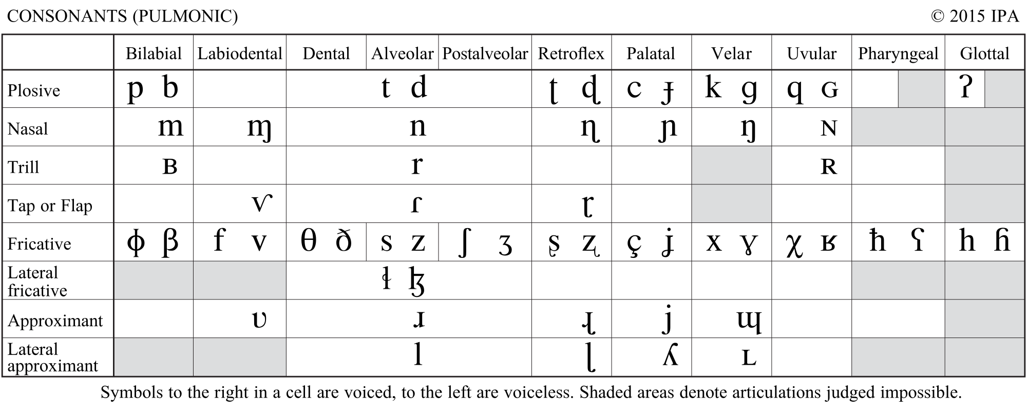
Figure 2.3: Table of consonants according to the manner (in rows) and place (in columns) of articulation. Figure from the International Phonetic Association (2015) - IPA Chart, available under a Creative Commons Attribution-Sharealike 3.0 Unported License.
To sum up, besides being an essential communication tool for humans, speech production is also a complex motor action, involving the fine-grained coordination of numerous laryngeal and supralaryngeal structures. In the next section, we discuss in more details the specific facial muscles that were of interest in the present work.
2.1.2 Orofacial speech muscles
In our work, we were especially interested in the activity of some of the orofacial muscles (i.e., the muscles situated around the mouth). More precisely, we studied the activity of the orbicularis oris inferior (OOI), the orbicularis oris superior (OOS), and the zygomaticus major (ZYG) muscles (cf. Figure 2.4). Contrary to what was assumed until recently, the orbicularis oris muscle is not a sphincter muscle but is instead a complex of several distinct muscles that interlace in a way that gives the orbicularis oris complex its circular aspect. Among these muscles, the OOS and the OOI are placed above and below (respectively) the mouth and are responsible for rounding or protruding the lips. The ZYG muscle has its origin on the zygomatic bone and inserts at the labial commissure (the angle of the mouth) where it meets with fibers of the levator anguli oris and orbicularis oris muscles. Together with the levator anguli oris, it serves to move the labial commissure upwards and laterally, and is involved in laughing and more generally in pleasant reactions and positive emotions. It is also involved in speech production, especially during the production of spread sounds, that is, sounds that require a wide horizontal aperture of the mouth (e.g., /i/).
Figure 2.4: Illustration of the main facial muscles of interest in the present work. Figure adapted from Patrick J. Lynch, medical illustrator, http://patricklynch.net.
For sensors placement, we followed guidelines and recommendations from Fridlund & Cacioppo (1986). In addition to speech-related orofacial muscles, we also routinely recorded the activity of other facial muscles such as the frontalis muscle (FRO) in Chapter 3, 4, 5, and the corrugator supercilii muscle (COR) in Chapter 5. The activity of these muscles was monitored to control for non speech-related facial muscular activity (as recommended by Garrity, 1977).
There are several ways to probe the involvement of specific articulators in a given speech production task. For instance, it is possible to selectively interfere with the activity of some articulators (or groups of articulators) to demonstrate their necessary involvement in this particular task. It is also possible to record the activity of facial muscles peripherally using surface electromyography, without interfering with (or with minimal interference to) the natural course of the speech production process. In the next section, we briefly introduce some core concepts of electromyography.
2.2 A brief introduction to electromyography
Technically speaking, electromyography (EMG) is a technique concerned with the recording and analysis of myoelectric signals (i.e., signals resulting from physiological variations in the state of muscle fibers membranes). Broadly speaking, EMG is a measure of the electrical activity generated during muscle contraction. It is used both as a basic tool in (for instance) biomechanical and psychophysiology research and as an evaluation tool in applied research (e.g., physiotherapy, rehabilitation, human-computer interfaces). To facilitate the interpretation of the EMG signal, it is useful to briefly detail the meaning of its physiological components.
2.2.1 Nature of the EMG signal
2.2.1.1 Muscular anatomy and physiology
A muscle is a collection of fibers that can vary in length, orientation, diameter, and architectural characteristics. For instance, deeper muscle fibers are usually composed of a greater proportion of slow-twitch fibers (type I muscle fibers) whereas more superficial muscle fibers comprise a greater proportion of larger and fast-twitch fibers (type II muscles fibers, Kamen & Gabriel, 2010). On the basis of their structure and contractile properties, we can identify three types of muscle tissues: i) the skeletal muscles are attached to bones, their function is to produce voluntary movements and to protect the organs, ii) the cardiac muscles, whose function is to pump blood and iii) the smooth muscles, involved in involuntary movements (e.g., respiration, moving food).
The contraction of the skeletal muscles is initiated by electrical impulses that propagate from the central nervous system to the muscle via the \(\alpha\)-motoneurons. Many (both larger and smaller) muscles are partitioned, with each portion having a specific role for the muscle function. Moreover, there is no one-to-one mapping between populations of motor neurons and muscle compartments. In other words, one population of motoneurons may innervate several compartments and reciprocally, several populations of motoneurons may innervate the same muscle compartment. Therefore, interpreting the EMG signal requires to be aware whether the recorded signal is characteristic of a whole muscle’ activity or of a specific muscle compartment (Kamen & Gabriel, 2010).
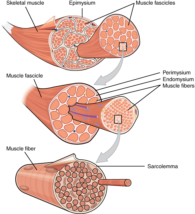
Figure 2.5: Structure of a skeletal muscle, muscle fascicle and muscle fiber. Figure from the OpenStax Textbook. Download for free at .
The muscle fiber is surrounded by a membrane, the sarcolemma (see Figure 2.5). Under resting conditions, the voltage inside the membrane is around -90mV, relative to the outside. This voltage results from a particular combination of sodium (\(\text{Na}^{+}\)), potassium (\(\text{K}^{+}\)), chloride (\(\text{Cl}^{-}\)), and other anions. At rest, the concentration of \(\text{Na}^{+}\) is relatively high outside the membrane and relatively low inside the membrane. The concentration of \(\text{K}^{+}\) follows an opposite pattern, with a greater concentration inside the membrane, and a lower concentration outside the membrane.
2.2.1.2 The motor action potential
Because muscle membranes can change their electrical state, muscle fibers are excitable tissues. When a muscle fiber is depolarised, the membrane potential produces a response called the muscle fiber ation potential or more generally the motor action potential (MAP). The generated action potential proceeds along the muscle fiber in both directions from the neuromuscular junction (Kamen & Gabriel, 2010).20 In the first phase of the MAP, the \(\text{Na}^{+}\) permeability increases dramatically, inducing a massive income of \(\text{Na}^{+}\) into the cell. This results in a temporary inversion of the cell polarity (see Figure 2.6).
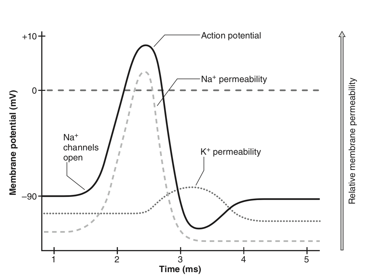
Figure 2.6: Time course of a motor action potential (figure from Kamen & Gabriel, 2010).
The MAP is followed by a refractory period, characterised by a decrease in membrane excitability. This refractory period can be further decomposed in an absolute refractory period during which all \(\text{Na}^{+}\) channels are closed, and a relative refractory period where some \(\text{Na}^{+}\) channels are open (but to a lesser extent than before the MAP). Interestingly, this after-impulse hyperpolarisation limits the frequency of MAPs (Kamen & Gabriel, 2010).
2.2.1.3 The motor unit
The motor unit is the smallest controllable muscular unit. It consists in a single \(\alpha\)-motoneuron, its neuromuscular junction, and all the muscle fibers it innervates. The number of motor units and their innervation ratio (i.e., the number of muscle fibers per motor unit) can vary by muscle. Because a single motoneuron can innervate multiple muscle fibers, the firing of a single motoneuron results in the simultaneous discharge of many muscle fibers. The motor unit action potential (MUAP) is the electric field resulting from the sum of the electric fields emitted by each fiber of the motor unit. In other words, it represents the spatiotemporal summation of individual MAPs originating from muscle fibers that are sufficiently close to a given electrode. This generates a train of MUAPs, called motor unit action potential trains (MUAPTs). The mixture of MUAPTs coming from different motor units constitute the raw EMG signal (cf. Figure 2.7).
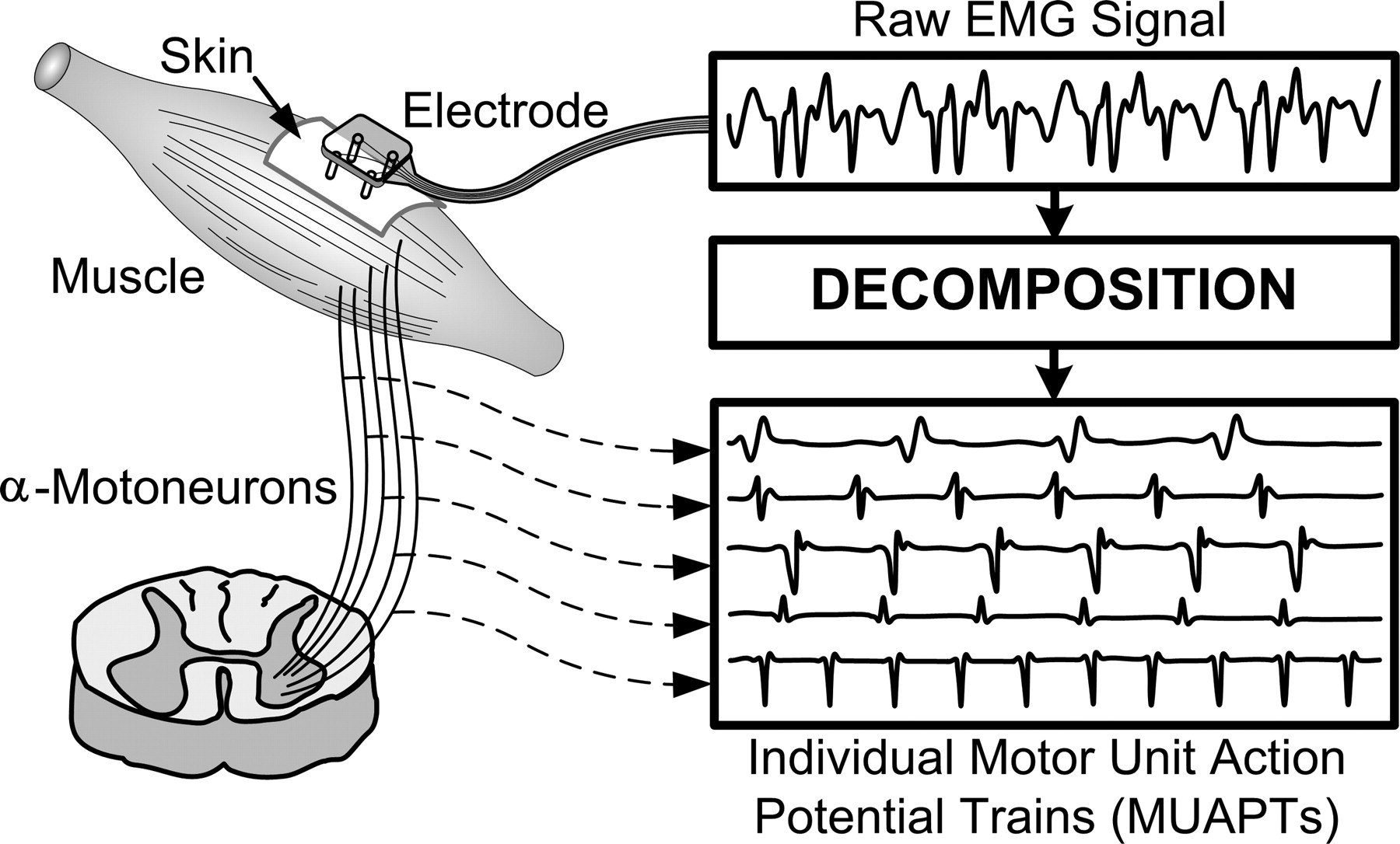
Figure 2.7: Motor unit action potential representation (figure from De Luca et al., 2006).
To sum up, the EMG signal results from a mixture of recruited motor units: it is composed of the sum of several to many MUAPTs. This signal can vary considerably because of factors such as the muscle length (Babault, Pousson, Michaut, & Van Hoecke, 2003), the distance between the muscle fiber (of interest) and the electrode, the fiber length or the muscle temperature. In the next section, we discuss in more details how this signal can be acquired.
2.2.2 EMG instrumentation and recording
Myoelectric measurements have a long history, starting in the XVII and XVIII centuries with the classical observations that muscle contraction can generate electricity and that electrical impulses can generate muscle contraction. The term of electromyography and the first EMG measures were realised at the end of the XIXth century, and the quality of EMG measurements did not cease to improve since (see Raez, Hussain, & Mohd-Yasin, 2006, for a brief historical perspective).
Two main types of sensors have been used to record EMG signals, varying by their invasiveness. First, indwelling (intramuscular) recordings can be acquired via electrodes directly inserted into the muscle. This form of EMG is mostly used in rehabilitation, for diagnosis of muscle function and to examine nerve conduction (Fridlund & Cacioppo, 1986). Second, surface electromyography can be recorded at the surface of the skin. Each method is associated with its own type of sensors, its own advantages and disadvantages. Surface electrodes have the advantage of being easy to use and non-invasive. However, their use is limited to (large and) superficial muscles. Moreover, because of the phenomenon of cross-talk,21 it is difficult to isolate the activity of specific muscles using surface EMG. On the opposite, intramuscular EMG (that can be recorded via a single needle or two wires implanted directly into the muscle) are highly selective and can sometimes record the activity of individual motor units. In addition, indwelling recordings are not submitted to tissue filtering (i.e., the fact that muscles tissues act as low-pass filters), in contrast to surface recordings.
Because of the important crossing and superposition of facial muscles, surface EMG recorded over facial muscles does not generally represent the activity of a single muscle, but rather a mixture of muscle activations (De Luca, 1997; Rapin, 2011). As a result, it is usually inappropriate, when using surface EMG, to attribute the recorded activity to a single muscle (Fridlund & Cacioppo, 1986). Whereas for the sake of simplicity, we designate sensors by the name of the underlying muscle of interest (e.g., “FRO” for the frontalis muscle), it should be kept in mind that these sensors reflect the activity of “sites”, rather than the activity of single muscles.
Aside from cross-talk, many other factors can affect the EMG signals. These factors are usually described under three main categories (for more details, see De Luca, 1997):
The causative factors, that have a basic effect on EMG signals. These factors can be further subdivided into two classes: i) the extrinsic factors, including factors such as the type of electrode (e.g., size, shape, placement) or the inter-electrode distance and ii) the intrinsic factors such as physiological or anatomical factors (e.g., fiber type, fiber diameter, blood flow).
The intermediate factors. These are the physiological phenomena that are influenced by one or more of the causative factors and that in turn influence the deterministic factors, such as the conduction velocity, spatial filtering or the signal cross-talk.
Finally, the deterministic factors are influenced by the intermediate factors and have a direct effect on the EMG signal. These include the number of active motor units or the amplitude, duration and shape of the MUAPs.
All these factors contribute to modulating both the amplitude of the EMG signal and its spectral properties (e.g., its mean or median frequency). The importance of these perturbating factors should be acknowledged and controlled as far as possible. In our work, we use a state-of-the art surface EMG apparatus, specifically developed to tackle these issues, as well as standardised procedures (more details regarding the EMG apparatus are provided in Chapters 3 to 5).
2.2.3 EMG signal processing
The raw EMG signal is a stochastic train of MUAPs. As put by Fridlund & Cacioppo (1986), “when heard through a speaker, the raw EMG signal sounds like popcorn popping”. Therefore, it is usually unsuitable for immediate quantification. In order to illustrate what the EMG signal looks like, we simulated EMG data based on a standard algorithm implemented in the biosignalEMG package (Guerrero & Macias-Diaz, 2018). This simulated EMG signal is represented in Figure 2.8.
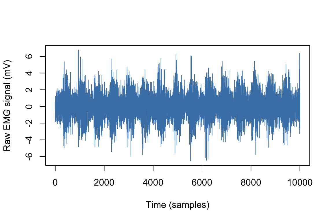
Figure 2.8: Simulated EMG signal.
We usually rectify the EMG signal by taking its absolute value and subtracting the mean in order to correct for any offset (bias) present in the raw data. The result of this operation is represented in Figure 2.9.
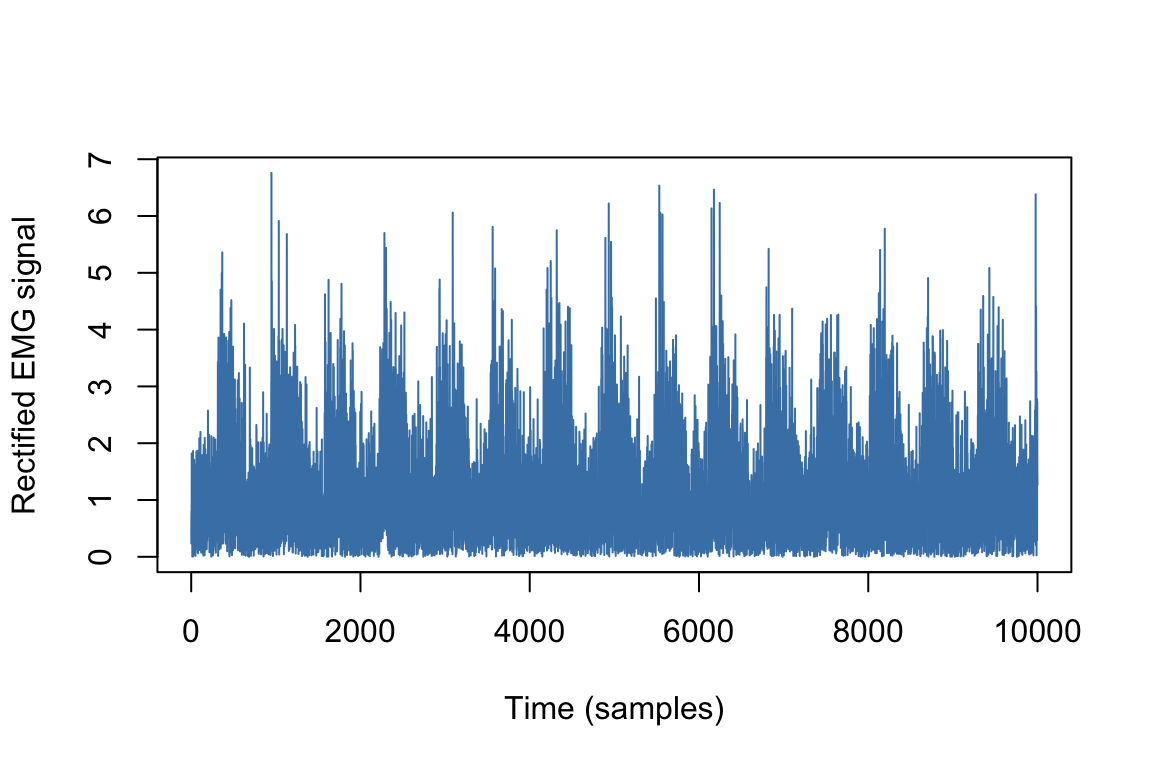
Figure 2.9: Rectified EMG signal.
Then, the signal is usually low-pass filtered, with a cut-off frequency depending on the nature of the study. From there, two main measures can be used to represent the magnitude of the muscle activity.22 The first one is the mean absolute value (MAV), which is computed over a specific interval of \(N\) samples. Its formula is given below, where \(|x_{n}|\) is the absolute value of an EMG sample in the data window.
\[MAV = \frac{1}{N} \sum_{n=1}^{N} | x_{n} |\]
The unit of measurement is usually the \(mV\) and the MAV calculation is generally similar to the numerical formula for integration (Kamen & Gabriel, 2010). The second one is the root-mean-square (RMS) amplitude:
\[RMS = \sqrt{ \frac{1}{N} \sum_{n=1}^{N} x^{2}_{n} }\]
where \(x^{2}_{n}\) is the squared value of each EMG sample and has both physical and physiological meanings. Put broadly, the RMS it taken to reflect the level of the physiological activities in the motor unit during contraction. Both the MAV and the RMS are illustrated in Figure 2.10.
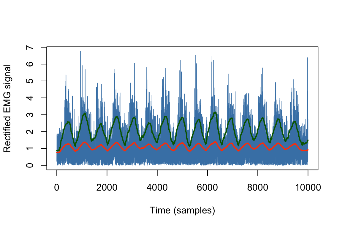
Figure 2.10: Illustration of the MAV (in orange) and RMS (in green) values. These two features are usually highly correlated but differ in magnitude. More precisely, the RMS is proportional to the MAV when the signal has a Gaussian shape.
These features provide the envelope of the rectified EMG signal. This envelope can then be summarised (e.g., via its mean or median) over a period of interest (e.g., during the utterance of some phoneme).
2.3 Statistical modelling and statistical inference
2.3.1 Limitations of the standard statistical approach in Psychology
Numerous authors have highlighted the limitations inherent to the Null-Hypothesis Significance Testing (NHST) approach and the (exclusive) reliance on p-values and significance testing (e.g., Bakan, 1966; Gigerenzer, 2004; Kline, 2004; Lambdin, 2012; Meehl, 1967; Trafimow et al., 2018). Considering these limitations, some authors have recommended to push away significance testing and to develop the use of effect size estimates and confidence intervals in order to favour accumulation of evidence and a meta-analytical mode of thinking (e.g., Cumming, 2012, 2014).
However, the apparent superiority of confidence intervals over p-values is an illusion. Indeed, as noted by many observers, confidence intervals are simply inverted significance tests. In other words, the confidence interval represents the range of values that are significant at some \(\alpha\) level. Therefore, compared to a p-value, a confidence interval does not bring any new inferential value. Moreover, its interpretation might be as hard as the interpretation of p-values. For instance, contrary to a widely shared belief, confidence intervals do not contain the \((1 - \alpha) \cdot 100\)% most probable values of the parameter (e.g., Morey, Hoekstra, Rouder, Lee, & Wagenmakers, 2015; Nalborczyk et al., 2019b).
That being said, it is fair to acknowledge that using confidence intervals (instead of or in addition to single p-values) does shift the emphasis from a mechanical (mindless) point-hypothesis testing procedure to a more careful consideration of the range of values that are compatible with some hypothesis. More importantly, it emphasises the uncertainty that accompanies every statistical procedure. Indeed, we think that most of the caveats that are attributed to a specific statistical procedure (e.g., to NHST) are really caveats of the way it is used. Namely, the fact that it is used in a categorical and absolute way. This tendency has been coined as dichotomania (i.e., the tendency to consider that results are either present –if significant– or absent –if non-significant), or trichotomania (e.g., when considering evidence ratios thresholds).
These biases have been highlighted by many statisticians in the past (e.g., Wasserstein & Lazar, 2016). Very recently, The American Statistician published a special issue on Moving to a World Beyond “p<.05”, with the intention to provide new recommendations for users of statistics (e.g., researchers, policy makers, journalists). This issue comprises 43 original papers aiming to provide new guidelines and practical alternatives to the “mindless” use of statistics. In the accompanying editorial, Wasserstein, Schirm, & Lazar (2019) summarise these recommendations in the form of the ATOM guidelines: “Accept uncertainty. Be thoughtful, open, and modest.” We describe below how our statistical approach might be understood in light of these core principles.
Accept uncertainty: we try to represent and to acknowledge uncertainty in our analyses and conclusions. For instance, we do not conclude and/or infer that an effect is either “present” or “absent”, but we report the estimated magnitude of the effect and the uncertainty that comes with this estimation. Additionally, when relevant, we report probabilistic statements based on the posterior distribution.
Be thoughtful: for each analysis opportunity (i.e., for each dataset to analyse), we consider what would be the most appropriate modelling strategy but we also acknowledge that there is no unique best way to analyse a given dataset. In most empirical chapters, we clearly distinguish between confirmatory (preregistered) and exploratory (non-preregistered) statistical analyses. We routinely evaluate the validity of the statistical model (and of its assumptions) and we are suspicious of statistical defaults. We try to consider the practical significance of the results, rather than their statistical significance. We use a variety of statistics (e.g., effect sizes, interval estimates, information criteria) to obtain a more diverse picture of the meaning of the results.
Be open: the soundness of a statistical procedure (and more generally, of an inferential procedure) can only be evaluated if it is made transparent to peers and readers for critical examination. Therefore, we take some space in the next section (but also in each experimental chapter) to motivate our statistical modelling decisions. We also make all
Rscripts available to ensure the reproducibility of the analyses. We try to be exhaustive in the way we report our analyses and we beware of shortcuts than could hinder important information to the reader.Be modest: we recognise that there is no unique “true statistical model” and we discuss the limitations of our analyses and conclusions. We also recognise that scientific inference is much broader than statistical inference and we try not to conclude anything from a single study without the warranted uncertainty.
To sum up, we try to acknowledge the uncertainty that accompanies every (statistical) inference. In the next section, we present in more details what our approach does entail and we introduce some key technical concepts.
2.3.2 Our statistical approach
In brief, we tried to move from the point-hypothesis mechanical testing to an approach that emphasises parameter estimation, model comparison, and continuous model expansion (e.g., Cumming, 2012, 2014; Gelman et al., 2013; Gelman & Hill, 2006; Judd, McClelland, & Ryan, 2009; Kruschke, 2015; Kruschke & Liddell, 2018a, 2018b; McElreath, 2016a). In other words, our approach can be defined as a statistical modelling approach rather than a statistical testing approach. It means that we try to model the data (or rather the process that generated the data), rather than to “test” it. We carefully consider what could be the process that generated the data and we try to model it appropriately. For instance, we do not fit reaction time data, Likert data, or electromyographic data using the same model, as this practice would lead to high rates of erroneous inferences.
Throughout this work, we use Bayesian statistical modelling, not by dogmatism, but because we think the Bayesian approach provides richer inferences than the frequentist one. The main advantage of the Bayesian approach is the explicit use of probability to model the uncertainty (see Box ). By doing so, the Bayesian approach permits to evaluate the probability of a parameter (or a vector of parameters) \(\theta\), given a set of data \(y\):
\[p(\theta|y) = \frac{p(y|\theta)p(\theta)}{p(y)}\]
Using this equation (known as Bayes’ theorem), a probability distribution \(p(\theta|y)\) can be derived (called the posterior distribution), that reflects knowledge about the parameter, given the data and the prior information. This distribution is the goal of any Bayesian analysis and contains all the information needed for inference.
The term \(p(\theta)\) corresponds to the prior distribution, which specifies the prior information about the parameters (i.e., what is known about \(\theta\) before observing the data) as a probability distribution. The left hand of the numerator \(p(y|\theta)\) represents the likelihood, also called the sampling distribution or generative model, and is the function through which the data affect the posterior distribution. The likelihood function indicates how likely the data are to appear, for each possible value of \(\theta\). Finally, \(p(y)\) is called the marginal likelihood. It is meant to normalise the posterior distribution, that is, to scale it in the “probability world”. It gives the “probability of the data”, summing over all values of \(\theta\) and is described by \(p(y) = \sum_{\theta} p(\theta) p(y|\theta)\) for discrete parameters, and by \(p(y) = \int p(\theta) p(y|\theta) d\theta\) in the case of continuous parameters.
All this pieced together shows that the result of a Bayesian analysis, namely the posterior distribution \(p(\theta|y)\), is given by the product of the information contained in the data (i.e., the likelihood) and the information available before observing the data (i.e., the prior). This constitutes the crucial principle of Bayesian inference, which can be seen as an updating mechanism. To sum up, Bayes’ theorem allows a prior state of knowledge to be updated to a posterior state of knowledge, which represents a compromise between the prior knowledge and the empirical evidence.
We also use multilevel models (also known as mixed-models) to handle complex dependency structures and to obtain more precise estimates. A more accurate description of Bayesian multilevel models is outside the scope of this introductory section but the interested reader is redirected toward several existing tutorial papers (e.g., Nalborczyk et al., 2019a; Nicenboim & Vasishth, 2016; Sorensen, Hohenstein, & Vasishth, 2016) or Appendix A. Throughout this work, we also make use of several tools with very distinct properties and uses. For instance, we use Bayes factors (BFs) to quantify the relative evidence for a statistical hypothesis (see Box ), we use information criteria to assess the predictive abilities of our models (see Box ), we use posterior predictive checks as well as a diagnostics tools (e.g., convergence indexes, trace plots) to assess the validity of our models, and we use summary statistics when appropriate to convey the meaning of the main results.
Bayes factors are often said to have desirable asymptotic (i.e., when the number of observations is very large) properties. Indeed, they are consistent for model identification. It means that if a “true” statistical model is in the set of models that are compared, using a BF will usually lead to selecting this “true” model with a probability approaching 1 with increasing sample size. Whether this seems an appealing property or not depends on the underlying statistical philosophy. Indeed, one could question whether it is sensible to assume a “true model” (an oxymoron) in real life, especially in the social sciences (e.g., Burnham & Anderson, 2002, 2004). As Findley (1985) notes: “[…] consistency can be an undesirable property in the context of selecting a model”. A more realistic question is then not to look for the “true” model, but rather for the best model for some practical purpose.
The usefulness of information criteria comes from them being approximations of the out-of-sample deviance (see Box ). In the present work, we used generalisations of the AIC (especially the WAIC and LOOIC) that also approximate the out-of-sample deviance and as such give an indication of how good/bad a model is to predict future (i.e., non-observed) data.
In brief, in the present work, we used various methods but coherently with a few (nuanced) guiding principles. Namely, we favoured a model comparison approach (e.g., Burnham & Anderson, 2002, 2004; Judd et al., 2009), we used several statistics when they provide complementary information (e.g., using both posterior probabilities, information criteria or BFs), we assessed the validity of our models (e.g., via posterior predictive checks), we reported these analyses transparently, and we tried to convey uncertainty in our conclusions.
2.4 Overview of the following chapters
The experiments carried out during this PhD will be presented as five empirical chapters that can be grouped under two main axes. In the first couple of experiments, we used surface electromyography and muscle-specific relaxation to investigate the involvement of the speech motor system during induced verbal and non-verbal rumination (Chapter 3 & 4). In Chapter 5, we used surface electromyography and machine learning algorithms to decode the muscle-specific EMG correlates of inner speech production. In the last couple of experiments, we switched strategy from the “correlates strategy” to the “interference strategy”, where the goal was to directly interfere with the activity of the speech motor system. More precisely, we used articulatory suppression to disrupt induced rumination in Chapter 6, and we used articulatory suppression to disrupt either induced rumination or problem-solving in Chapter 7. Finally, in Chapter 8, we summarise the main findings, discuss their implications and suggest ways forward from both a theoretical and an experimental perspective.
The neuromuscular junction is the site where the motoneuron meets the muscle fiber.↩
The phenomenon of cross-talk can be defined as the mixing of the electrical activity of the muscle of interest with the electrical activity of adjacent or distant muscles, that are not of primary interest.↩
But see for instance Phinyomark, Nuidod, Phukpattaranont, & Limsakul (2012), for a brief overview of other features that can be extracted from the surface EMG signal.↩